side channels: power analysis
This is a post in a serie regarding side channels, from the theoretical and pratical point of view; the posts are
- introduction on the model of computing devices (to be finished)
- using the Chipwhisperer (here)
- power analysis (this post)
- glitching (to be finished)
All the graphs in this post are generated using my own libray named power_analys, this is alpha-quality software without documentation (for now); also a notebook with all the code that generated the graphs will be available as soon as I take the time to clean up it.
Physical interface
As I said in the (to-be-completed) post about the model of a processing unit, the "calculations" inside a device are done, roughly speaking, switching on and off groups of transistors to perform the needed operations; since the transistors are physical entities, they interact with the physical world and need energy to move electrons around, so we can imagine that the power consumption would be in some way connected with the internal state of the processor1.
To measure the power consumption, tipically you have a shunt resistor between the
power line and the VCC pin of the target with an ADC measuring the voltage as indicated in the
drawing below

this works because thanks to Ohm's law, the voltage difference at the sides of the resistor is proportional to the current drawn from the device.
In general it's possible that multiple pins are responsible for providing power to the digital device and maybe each pin serves different subsystems (peripherals, core, etc...), so in real settings the configuration can be more complex.
In my experiments I'm going to use the ChipWhisperer-lite, it has the
AD8331
chip (a variable gain amplifier, VGA) and the
AD9215
(an ADC). The target's clock and ADC are synchronized, only the latter
has a sample rate four times of the former (this ratio can be configured).
The configuration of the VGA is such that the input impedance is 50 ohm
(see table 7 at page 30 of the datasheet) and
AC-coupled (so you don't have DC component, at least theoretically); this explains why, since
the input is connected to the low side of the shunt resistor on the board, you
have negative readings: the high side is ideally constant (at the power
supply voltage) so, without AC-coupling you would obtain something like
$$ V_{L} = V_H - I\times R_\hbox{shunt} $$
but removing the constant voltage, what you see from the traces is
$$ \eqalign{ AC(V_{L}) &= AC(V_H) + AC(-I\times R_\hbox{shunt}) \cr &= AC(-I\times R_\hbox{shunt})\cr } $$
The actual value that you'll find in the traces are also affected by the
gain set for the VGA.
Note: the power consumption is not technically the values that you are capturing but has a direct relation with them: the textbook definition is
$$ P = V\cdot I $$
If the assumption is that the voltage is constant with a low-amplitube varying component (let's call it \(V_{AC}\)) we can obtain the following approximation
$$ \eqalign{ P &= V\cdot I \cr &= (V_{DC} + V_{AC})\cdot I \cr &= V_{DC}\left(1 + {V_{AC}\over V_{DC}}\right)\cdot I\cr &\sim V_{DC}\cdot I\cr } $$
that works fine as long as \({V_{AC}\over V_{DC}}\) is negligible. So at the end the amplitude measured is really, up to a constant, the power consumption.
Since we are not going to do real physics, for now this is enough to continue.
Maths&Statistics
To understand a little better what we are going to see in the following we need to have an overview of what we mean by correlation: what follows is an introduction of the statistical formalism needed to explain correlation power analysis2.
First of all, we need a model to describe the relationship between power consumption and the digital world: the simplest one with usefulness is the model using the Hamming weight or Hamming distance.
The Hamming weight is a quantity defined over a number using its base 2 representation: if \(d\) is a number such that
$$ d = \sum_{i=0}^{N - 1} d_i 2^i\hbox{ with }d_i\in \{0,1\} $$
we define the hamming weight as
$$ HW(d) = \sum_{i=0}^{N - 1} d_i $$
Although the Hamming weight is not linear with respect to its argument, if we see \(d\) as a uniformly independent random variable we can safely assume for the mean and variance for the Hamming weight
$$ \mu_H = {N\over 2}\qquad\sigma^2_H = {N\over4} $$
What does it mean? simply that when we are going to capture traces, we are going to feed as input random bytes (in statistical terms are random variables), since the HW inherits randomness from them, it's also treated as a random variable, allowing to use statistical tools to analyze the results.
Another important quantity related to the Hamming weight is the Hamming distance that measure the number of bit flip between two numbers (represented in base 2); this quantity as a very simple definition 3
$$ HD(S, D) = HW(S\oplus D) $$
where \(\oplus\) is the xor (exclusive or) operation defined via this
truth table
| A | B | A \(\oplus\) B |
|---|---|---|
| 0 | 0 | 0 |
| 0 | 1 | 1 |
| 1 | 0 | 1 |
| 1 | 1 | 0 |
An interesting property is its simmetry
$$ A\oplus B = B \oplus A $$
and interestingly, if we fix one operand and make the other a uniformly random independent variable, the Hamming distance has the same mean and variance as the Hamming weight. We will see later how this can be useful.
What we want to achieve is the "measure" of the correlation between our model's parameters and the power consumption and to do that we need to use the Pearson's correlation factor: its definition is given by
$$ \rho(A,B) = {Cov(A, B)\over\sigma_A\sigma_B} $$
where \(A\) and \(B\) are random variables; the value of \(\rho(A, B)\) is comprised between \(-1\) and \(1\), when two variables are independent \(\rho\) has a value of zero.
In the following experiments I'm going to use (implicitely) a model where the power consumption \(W\) is related to the Hamming weight of some input \(D\) (as a random variable) by the following relation
$$ W = aH(D) + b $$
where \(b\) is a noise term, all the contributions for the power consumption of the device not involved with the computation directly.
From this model is possible to obtain the following statistical relations:
$$ \eqalign{ \sigma^2_W &= a^2\sigma^2_H + \sigma^2_b\cr \rho(W, H) &= {Cov(W, H)\over\sigma_W\sigma_H}\cr &= {Cov(aH+b, H)\over\sqrt{a^2\sigma^2_H + \sigma^2_b}\sigma_H}\cr &= {aCov(H, H)\over\sqrt{a^2\sigma^2_H + \sigma^2_b}\sigma_H}\cr &= {a\sigma_H^2\over\sqrt{a^2\sigma^2_H + \sigma^2_b}\sigma_H}\cr &= {a\sigma_H\over\sqrt{a^2\sigma^2_H + \sigma^2_b}}\cr &= {a\sqrt{N/4}\over\sqrt{a^2{N/4} + \sigma^2_b}}\cr &= \hbox{sign}(a){\sqrt{N}\over\sqrt{N + 4\sigma^2_b}}\cr } $$
so the absolute value of the correlation tends to the limit of 1 when the noise term is negligible, where the sign is given only by the sign of the coefficient \(a\).
Another useful fact for later, related to the Hamming distance, is that if you want to maximise the correlation of this with respect to a fixed "background", this maximum is unique2.
Measuring different instructions
Before starting crunching numbers, a very simple overview of how different instructions have different "energy-footprint": let's try to show the power consumption of the target executing
- 10
nops - 10
muls - 20
muls - 10
muls, 10nops and 10muls
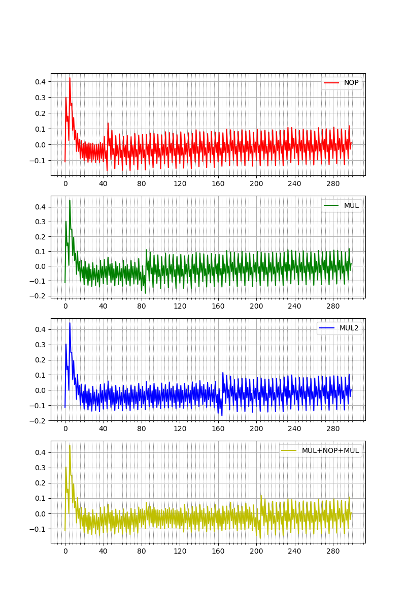
the assembly code is the following (each column is a different capture)
nop             mul r0, r1     mul  r0, r1     mul  r0, r1
nop             mul r0, r1     mul  r0, r1     mul  r0, r1
nop             mul r0, r1     mul  r0, r1     mul  r0, r1
nop             mul r0, r1     mul  r0, r1     mul  r0, r1
nop             mul r0, r1     mul  r0, r1     mul  r0, r1
nop             mul r0, r1     mul  r0, r1     mul  r0, r1
nop             mul r0, r1     mul  r0, r1     mul  r0, r1
nop             mul r0, r1     mul  r0, r1     mul  r0, r1
nop             mul r0, r1     mul  r0, r1     mul  r0, r1
nop             mul r0, r1     mul  r0, r1     mul  r0, r1
rjmp    .-2     rjmp    .-2    mul  r0, r1     nop
                               mul  r0, r1     nop
                               mul  r0, r1     nop
                               mul  r0, r1     nop
                               mul  r0, r1     nop
                               mul  r0, r1     nop
                               mul  r0, r1     nop
                               mul  r0, r1     nop
                               mul  r0, r1     nop
                               mul  r0, r1     nop
                               rjmp .-2        mul  r0, r1
                                               mul  r0, r1
                                               mul  r0, r1
                                               mul  r0, r1
                                               mul  r0, r1
                                               mul  r0, r1
                                               mul  r0, r1
                                               mul  r0, r1
                                               mul  r0, r1
                                               mul  r0, r1
                                               rjmp .-2
the tail of the capture is the rjmp instruction that loops indefinitely.
The big spike at the start of the capture is probably the current generated by
the GPIO used to trigger the capture.
The first thing that you can notice is that ten nops are taking 40 cycles to
complete (i.e. 10 target's clock cycles) meanwhile ten muls needs double
that number. This matches with the actual number of cycles needed by these
instructions: nop executes in one cycle, meanwhile mul takes two cycles
and each cycle the ADC samples four times.
Correlation
In the last section I showed that different instructions have different "footprints", probably the easiest possible way to use that is by timing analysis: for example if we had a piece of code that checks for a password and exits at the first wrong character, we could capture the power traces for every possible (first char) input and we should see only one having a different pattern.
What follows is an example with the firmware provided by the Chipwhisperer
(basic-passwdcheck) where the h character is the first of the secret
password (I grouped the traces in sets of 16 to make clearer the "outcast")
For now I'm not interested in performing specific attacks but to study the relationship between instructions and power consumption and to do this I will perform an "experiment" where I use as input the firmware code with the simplest possible assembly instructions.
The first experiment is to check what we can infer from the relation between the
argument of the instruction ldi r16, <value> and the power consumption: these
are the (interesting portion of) instructions (sts is the instruction
triggering the capture of the trace)
 6de:   c0 93 05 06     sts 0x0605, r28
 6e2:   00 00           nop
 6e4:   00 00           nop
 6e6:   00 00           nop
 6e8:   00 00           nop
 6ea:   00 00           nop
 6ec:   00 00           nop
 6ee:   00 00           nop
 6f0:   00 00           nop
 6f2:   00 00           nop
 6f4:   00 00           nop
 6f6:   00 e0           ldi r16, <value>
 6f8:   00 00           nop
 6fa:   00 00           nop
 6fc:   00 00           nop
 6fe:   00 00           nop
 700:   00 00           nop
 702:   00 00           nop
 704:   00 00           nop
 706:   00 00           nop
 708:   00 00           nop
 70a:   00 00           nop
 70c:   ff cf           rjmp    .-2
As you can see there is the instruction of interested sourrounded by input-independent code, this should make the relation standing out.
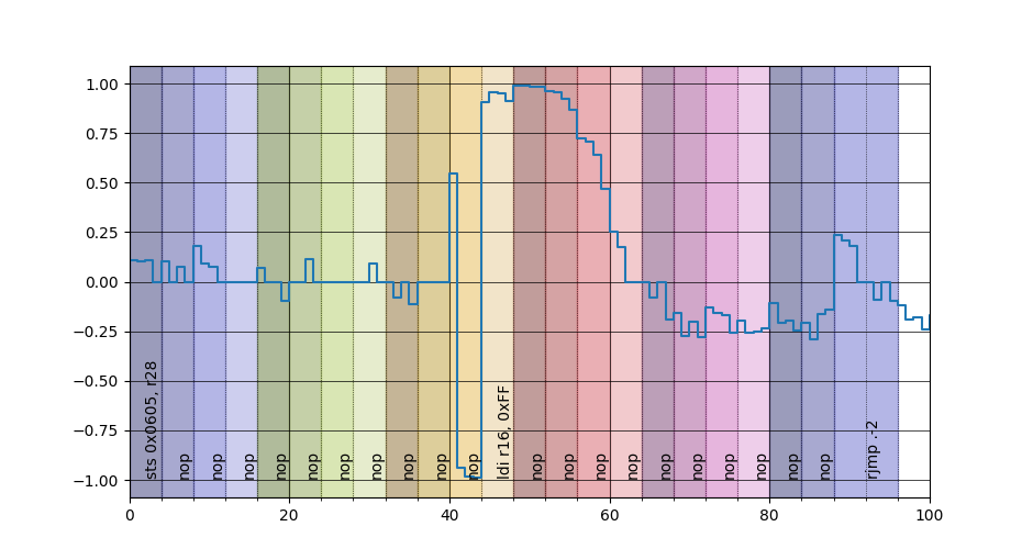
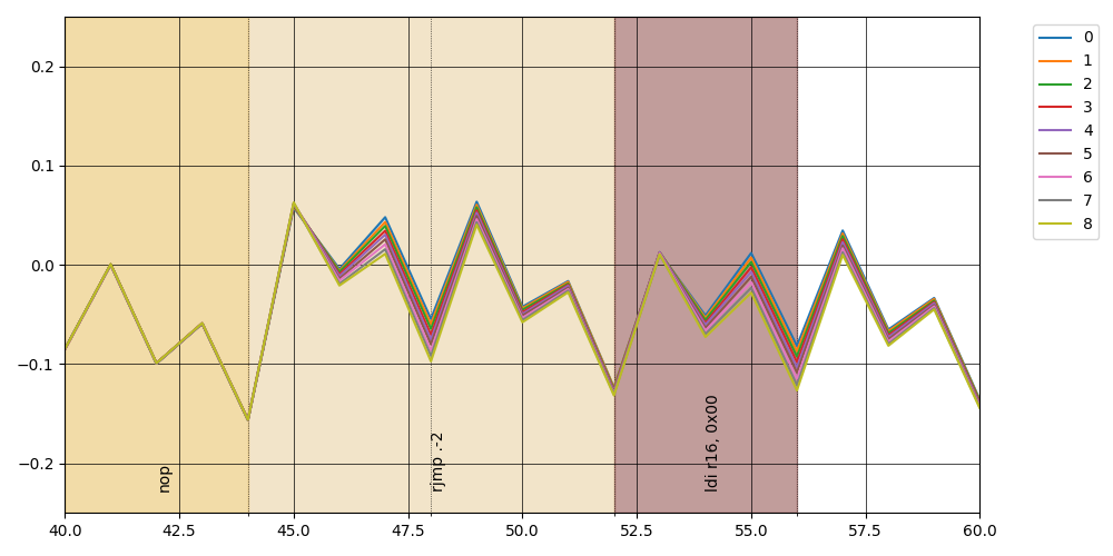
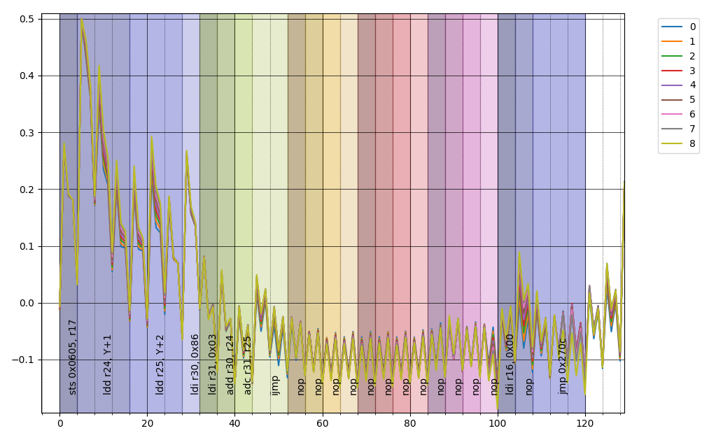
After capturing 100 traces for each hamming weight it's possible to plot the average for each one together as in the following plot where I tried to align the instructions with the actual clock cycle where they should happen (I'm not sure of the alignment of the trace with the actual instructions, so the instruction in picture are the first guess)
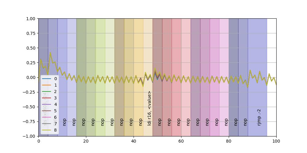
It's possible to note "something going on" around the ldi instruction; if
we zoom in we can see a little better
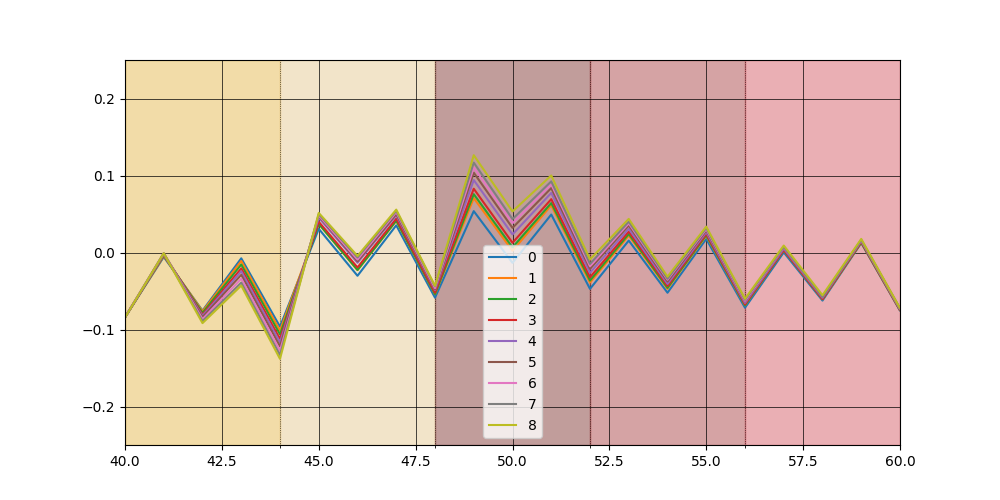
At first seems disaligned by half-instruction, take note of this for the following.
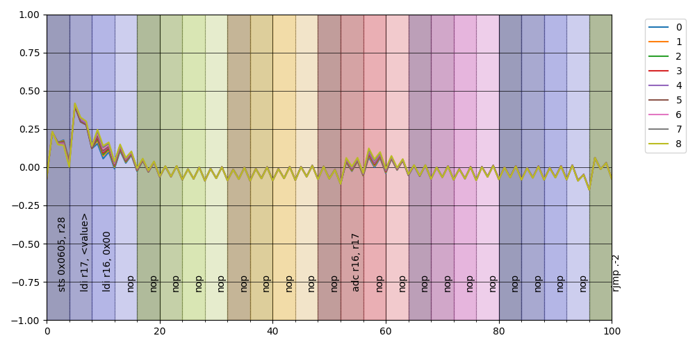
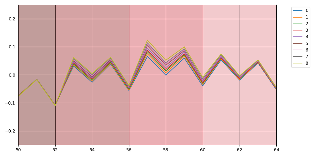
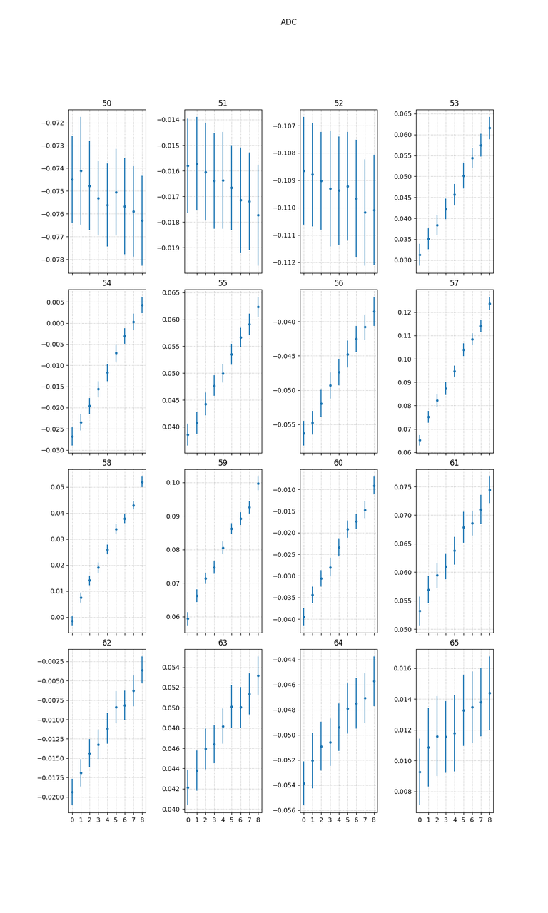
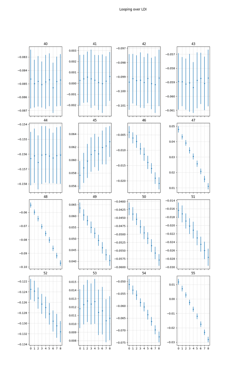
Meanwhile it's possible to have a better view plotting a scatterplot of mean value of a given sample for a specific Hamming weight versus the corresponding hamming weight (the vertical bars are the standard deviations of each respective set of traces):
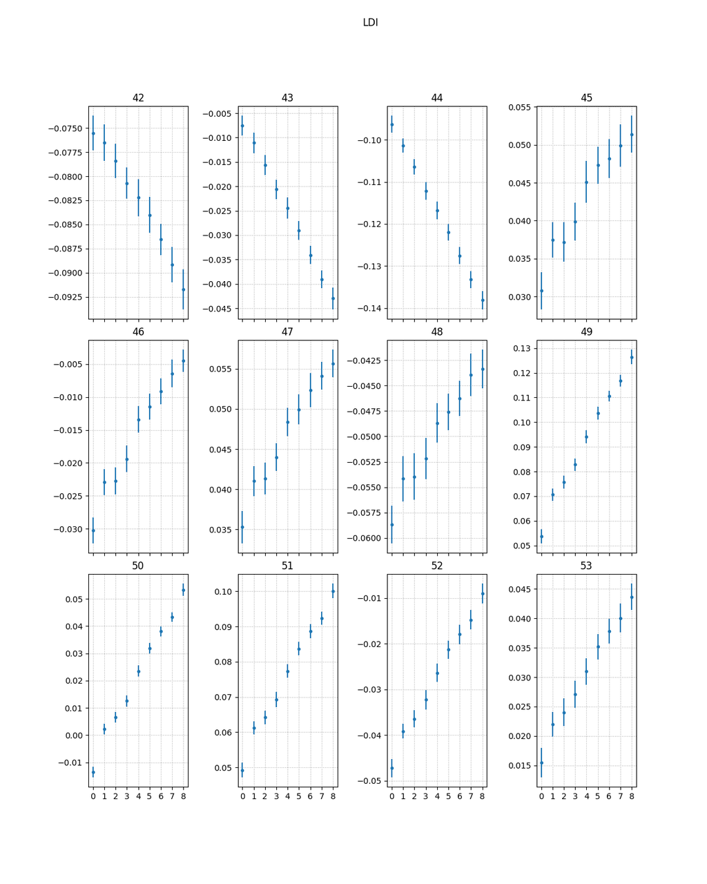
The first interesting samples have a negative correlation but after a couple of cycles this change to positive improving considerebly (note for example at sample 50 the standard deviations are way far from each other, this means that also taking noise into consideration the respective sets of traces are "separated").
The final graph is the correlation I talked so much about
Just with one kind of instruction is not possible to deduce anything valuable
(althought it's interesting seeing that something is there), now I want to try
a different instruction: adc rx, <value>.
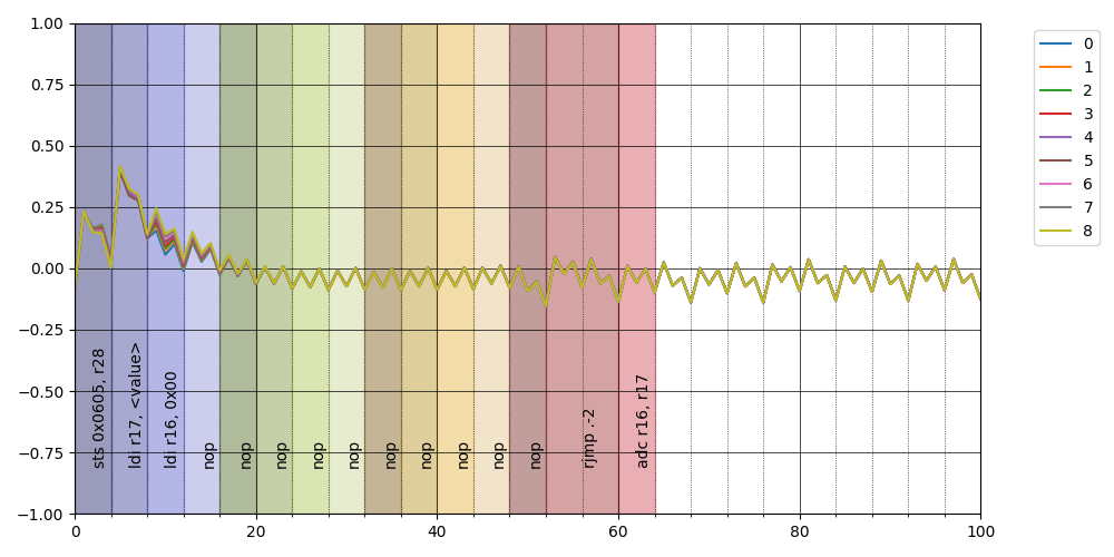
This is the code under scrutiny
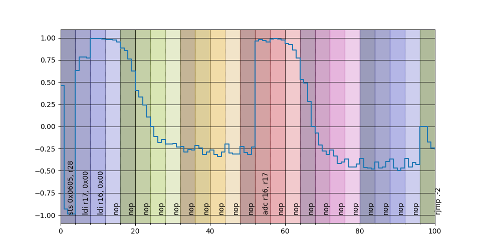
 6de:   c0 93 05 06     sts 0x0605, r28
 6e2:   10 e0           ldi r17, <value>
 6e4:   00 e0           ldi r16, 0x00
 6e6:   00 00           nop
 6e8:   00 00           nop
 6ea:   00 00           nop
 6ec:   00 00           nop
 6ee:   00 00           nop
 6f0:   00 00           nop
 6f2:   00 00           nop
 6f4:   00 00           nop
 6f6:   00 00           nop
 6f8:   00 00           nop
 6fa:   01 1f           adc r16, r17
 6fc:   00 00           nop
 6fe:   00 00           nop
 700:   00 00           nop
 702:   00 00           nop
 704:   00 00           nop
 706:   00 00           nop
 708:   00 00           nop
 70a:   00 00           nop
 70c:   00 00           nop
 70e:   00 00           nop
 710:   ff cf           rjmp    .-2
Plotting each averaged class we obtain something similar to before
but notice how the instructions seem aligned perfectly!
in particular is interesting to note that there is not in this case a negative correlation around the start of the instruction
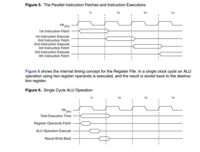
What explanation is available for this behaviour? Well, a modern processing unit employs some tricks to speed-up computation and a prevalent one is the pipeling, i.e., splitting the instruction life cycle in different stages and when the unit is executing a given instruction is also doing other stuff with the instruction that should be executed next; in particular for the XMega we have this quote from the manual:
The AVR uses a Harvard architecture - with separate memories and buses for program and
data. Instructions in the program memory are executed with a single level pipeline. While one
instruction is being executed, the next instruction is pre-fetched from the
program memory. This concept enables instructions to be executed in every clock cycle
To clarify a little better here a diagram
Now if you take a look at the AVR instruction set manual
you can see how the opcode for the ldi instruction is encoded:
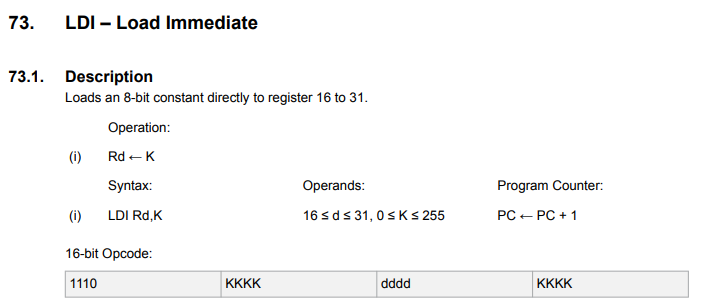
i.e. the value to put in the register is encoded directly in the instruction that is read in the fetching stage during the previous instruction!
With this in mind for now on I assume that the alignment is correct (another
implicit assumption is that the sts instruction, that is two-cycles long,
executes at the last cycle); while
I'm at it I want to double-proof the fetching stage assumption for ldi
putting an infinite loop just before it :)
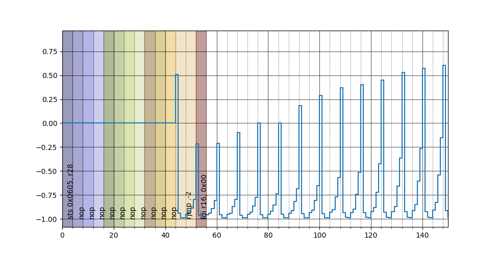
Observe what happens if we flash this code
 6de:   c0 93 05 06     sts 0x0605, r28 ; 0x800605 <__TEXT_REGION_LENGTH__+0x7de605>
 6e2:   00 00           nop
 6e4:   00 00           nop
 6e6:   00 00           nop
 6e8:   00 00           nop
 6ea:   00 00           nop
 6ec:   00 00           nop
 6ee:   00 00           nop
 6f0:   00 00           nop
 6f2:   00 00           nop
 6f4:   00 00           nop
 6f6:   ff cf           rjmp    .-2         ; 0x6f6 <main+0x56>
 6f8:   00 e0           ldi r16, <value>
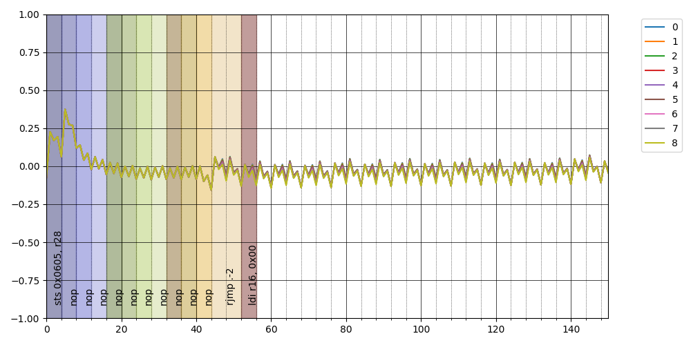
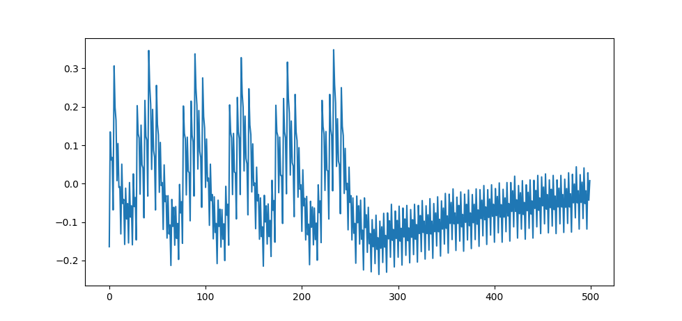
it's clearly visible a repeated pattern, look at this zoom
and the repeation in the correlation
Compare what you have seen with the same concept applied to the adc
No correlation at all! I mean, this would have been obvious from the start but it's always better to double check unexpected results :)
Now to improve on my experiment I decided to change strategy: until now I
flashed a different code every time I wanted to read a particular value for
ldi but this involves overwriting the flash so I decided to write some code
to build a jump table; with this code a character is read from the serial,
converted to an integer and used as an index to jump to a specific block where
the ldi r16, <value> is waiting to execute (I have a specific post about
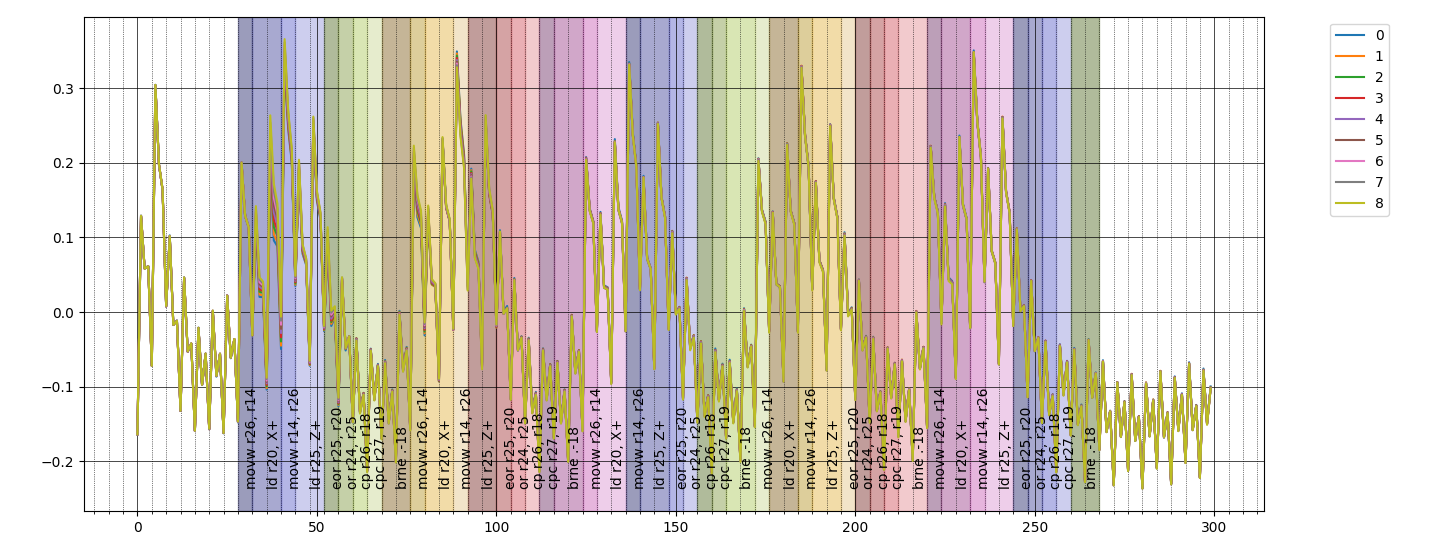
reversing AVR assembly if you want to understand what is happening).
and also in this case it's pretty amazing how the instructions align perfectly
(by the way, an old AVR instruction set manual indicated contradicting values for
the number of cycles for the ldd instruction so I used this captures as a
evidence for the correct number).
There is only one thing that bothers me, there is apparently a "tail" after the
instruction that shouldn't be there, my educated guess is that the ADC
frontend, being AC coupled causes this anomaly since the capacitor in front
of the measuring device has a change oscillating with the flow of current.
On order to test this I tried to capture the power consumption using my trusty Siglent using some python code that I wrote, but this is argument of a future post.
A more realistic case
Now I want to try to apply to the simplest difficult problem, i.e., trying to break a constant time password comparison; the code is the following
#define PASSWORD "kebab"
#define SIZE_INPUT 32

int main(void)
{

    char password[] = PASSWORD;

    platform_init();
    init_uart();
    trigger_setup();

    /* banner requesting the password */
    putch('p');
    putch('a');
    putch('s');
    putch('s');
    putch('w');
    putch('o');
    putch('r');
    putch('d');
    putch(':');
    putch(' ');

    /* taking the password, waiting for a newline or for SIZE_INPUT characters */
    char c;
    char input[SIZE_INPUT];
    unsigned int input_index = 0;

    do {
        c = getch();
        input[input_index++] = c;
    } while(c != '\n' && input_index < SIZE_INPUT);

    trigger_high();

    unsigned char result = 0;

    for (uint8_t index = 0 ; index < strlen(PASSWORD) ; index++) {
        result |= input[index] ^ password[index];
    }

    if (result)
        while(1);

    putch('W');
    putch('I');
    putch('N');

    while(1);
}
and this is the generated assembly (I advice always to check generated code because the compiler sometimes does magic)
000006c6 <main>:
 6c6:   cf 93           push    r28
 6c8:   df 93           push    r29
 6ca:   cd b7           in      r28, 0x3d       ; 61
 6cc:   de b7           in      r29, 0x3e       ; 62
 6ce:   a6 97           sbiw    r28, 0x26       ; 38 <--- allocate 38 byte on the stack (32 for the input, 6 for the hardcoded password (that includes the null byte))
 6d0:   cd bf           out     0x3d, r28       ; 61
 6d2:   de bf           out     0x3e, r29       ; 62
 6d4:   86 e0           ldi     r24, 0x06       ; 6  <--- set the counter to six
 6d6:   e0 e1           ldi     r30, 0x10       ; 16
 6d8:   f0 e2           ldi     r31, 0x20       ; 32 <--- set the source Z to the password
 6da:   de 01           movw    r26, r28             <--- set dest to X (on the stack)
 6dc:   91 96           adiw    r26, 0x21       ; 33 <--- with a starting offset of 33
 6de:   01 90           ld      r0, Z+               <---- loop starts here with r0 = *Z++
 6e0:   0d 92           st      X+, r0               <---- *(X++) = r0
 6e2:   8a 95           dec     r24                  <---- decrement counter
 6e4:   e1 f7           brne    .-8                  <---- jump if not zero -------
 6e6:   0e 94 4d 03     call    0x69a   ; 0x69a <platform_init>
 6ea:   0e 94 7c 02     call    0x4f8   ; 0x4f8 <init_uart0>
 6ee:   81 e0           ldi     r24, 0x01       ; 1
 6f0:   80 93 01 06     sts     0x0601, r24     ; 0x800601 <__TEXT_REGION_LENGTH__+0x7de601>
 6f4:   80 e7           ldi     r24, 0x70       ; 112
 6f6:   0e 94 b9 02     call    0x572   ; 0x572 <output_ch_0>
 6fa:   81 e6           ldi     r24, 0x61       ; 97
 6fc:   0e 94 b9 02     call    0x572   ; 0x572 <output_ch_0>
 700:   83 e7           ldi     r24, 0x73       ; 115
 702:   0e 94 b9 02     call    0x572   ; 0x572 <output_ch_0>
 706:   83 e7           ldi     r24, 0x73       ; 115
 708:   0e 94 b9 02     call    0x572   ; 0x572 <output_ch_0>
 70c:   87 e7           ldi     r24, 0x77       ; 119
 70e:   0e 94 b9 02     call    0x572   ; 0x572 <output_ch_0>
 712:   8f e6           ldi     r24, 0x6F       ; 111
 714:   0e 94 b9 02     call    0x572   ; 0x572 <output_ch_0>
 718:   82 e7           ldi     r24, 0x72       ; 114
 71a:   0e 94 b9 02     call    0x572   ; 0x572 <output_ch_0>
 71e:   84 e6           ldi     r24, 0x64       ; 100
 720:   0e 94 b9 02     call    0x572   ; 0x572 <output_ch_0>
 724:   8a e3           ldi     r24, 0x3A       ; 58
 726:   0e 94 b9 02     call    0x572   ; 0x572 <output_ch_0>
 72a:   80 e2           ldi     r24, 0x20       ; 32
 72c:   0e 94 b9 02     call    0x572   ; 0x572 <output_ch_0>
 730:   ce 01           movw    r24, r28
 732:   01 96           adiw    r24, 0x01       ; 1
 734:   7c 01           movw    r14, r24
 736:   8e 01           movw    r16, r28
 738:   0f 5d           subi    r16, 0xDF       ; 223 <--- r16 = fp - 32
 73a:   1f 4f           sbci    r17, 0xFF       ; 255
 73c:   6c 01           movw    r12, r24
 73e:   0e 94 b2 02     call    0x564   ; 0x564 <input_ch_0>
 742:   d6 01           movw    r26, r12
 744:   8d 93           st      X+, r24
 746:   6d 01           movw    r12, r26
 748:   8a 30           cpi     r24, 0x0A       ; 10
 74a:   19 f0           breq    .+6             ; 0x752 <main+0x8c>
 74c:   a0 17           cp      r26, r16
 74e:   b1 07           cpc     r27, r17
 750:   b1 f7           brne    .-20
 752:   81 e0           ldi     r24, 0x01       ; 1
 754:   80 93 05 06     sts     0x0605, r24
 758:   f8 01           movw    r30, r16        <--- Z points to password
 75a:   9e 01           movw    r18, r28
 75c:   2a 5f           subi    r18, 0xFA       ; 250
 75e:   3f 4f           sbci    r19, 0xFF       ; 255
 760:   80 e0           ldi     r24, 0x00       ; 0
 762:   d7 01           movw    r26, r14        <--- loop starts here
 764:   4d 91           ld      r20, X+
 766:   7d 01           movw    r14, r26
 768:   91 91           ld      r25, Z+
 76a:   94 27           eor     r25, r20
 76c:   89 2b           or      r24, r25
 76e:   a2 17           cp      r26, r18
 770:   b3 07           cpc     r27, r19
 772:   b9 f7           brne    .-18            ; 0x762 <main+0x9c>
 774:   81 11           cpse    r24, r1
 776:   ff cf           rjmp    .-2             ; 0x776 <main+0xb0>
 778:   87 e5           ldi     r24, 0x57       ; 87
 77a:   0e 94 b9 02     call    0x572   ; 0x572 <output_ch_0>
 77e:   89 e4           ldi     r24, 0x49       ; 73
 780:   0e 94 b9 02     call    0x572   ; 0x572 <output_ch_0>
 784:   8e e4           ldi     r24, 0x4E       ; 78
 786:   0e 94 b9 02     call    0x572   ; 0x572 <output_ch_0>
 78a:   ff cf           rjmp    .-2             ; 0x78a <main+0xc4>
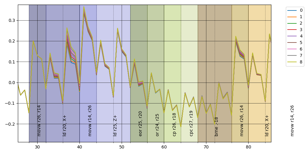
Let see a single capture
it's possible to deduce that there are five iterations happening before the infinite loop (five is the number of characters in the password).
Note: this could seem boring but for me it's very important: thanks to power analysis you have some sort of oracle that gives you information otherwise unavailable! Imagine you have a device that presents some sort of password prompt and you, via tinkering from the terminal can asses that accepts up to 32 characters; this means you have \(\left(2^8\right)^{32} = 2^{256}\) possible passwords, a key space huge, without hope to be bruteforced.
But from power analysis you have now reduced the key space to \(\left(2^8\right)^{5} = 2^{40}\) more feasible (an encryption algorithm with such "strength" would be considered broken). Obviously a 32 characters password doesn't have this problem :)
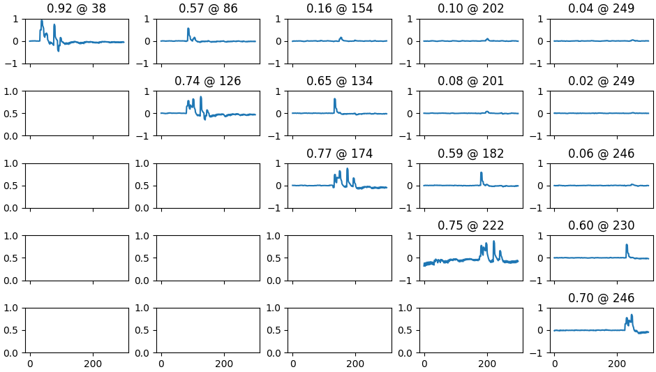
Now if we study only the power consumption in relation to the 0th byte of input it's possible to see "something happening" only in the first iteration of the loop (actually there is something going on also at the start of the second iteration, but "less").
here the zoom
This is interesting: we have a way to see when our input is used in the computation; in the graph above I overlayed the instructions but obviously in general this is not possible, however this temporal information instead is available via power analysis. This is akin to taint analysis done in security research were the software is analyzed to find how the user input can "propagate" and impact execution, take a look at libdft for example. But this out of scope (for now :P).
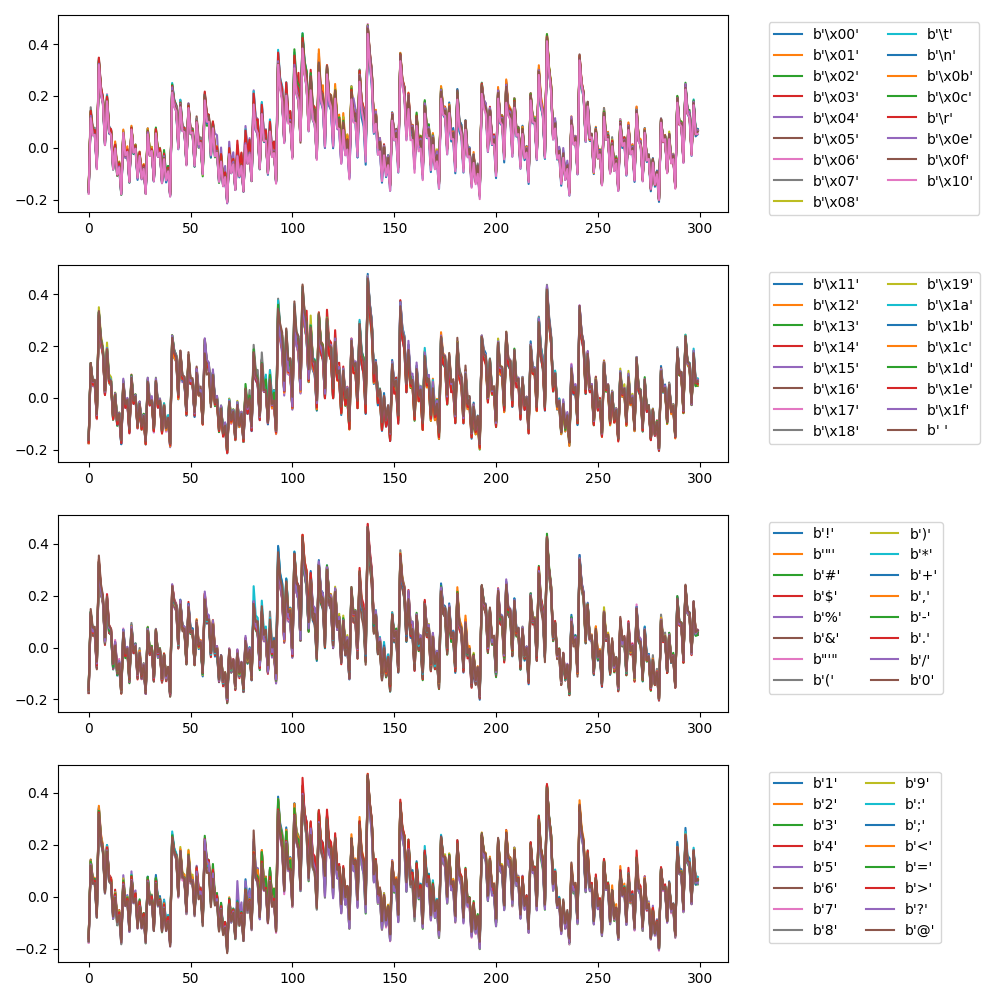
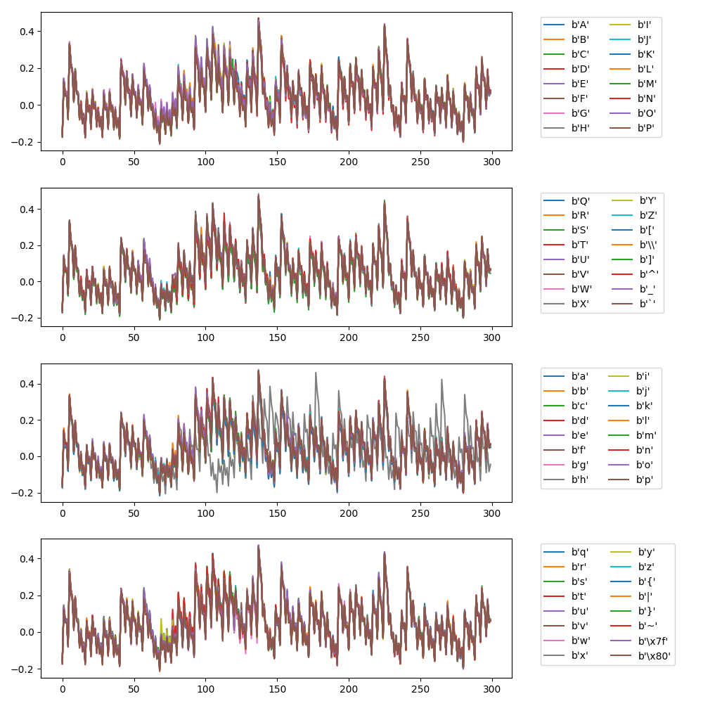
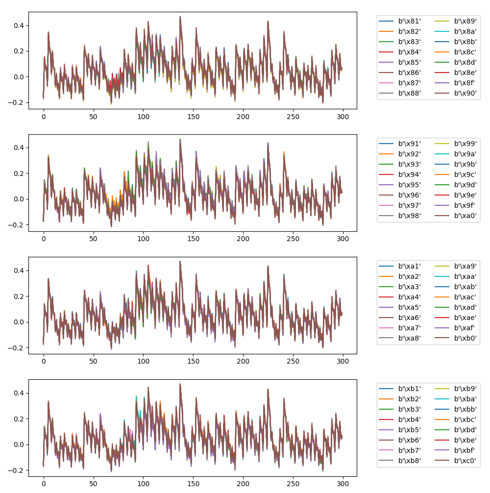
Now I want to try something new: remember the stuff above about the Hamming distance
and the xor operation? in
this case I want to try to find for each sample the element which xor creates
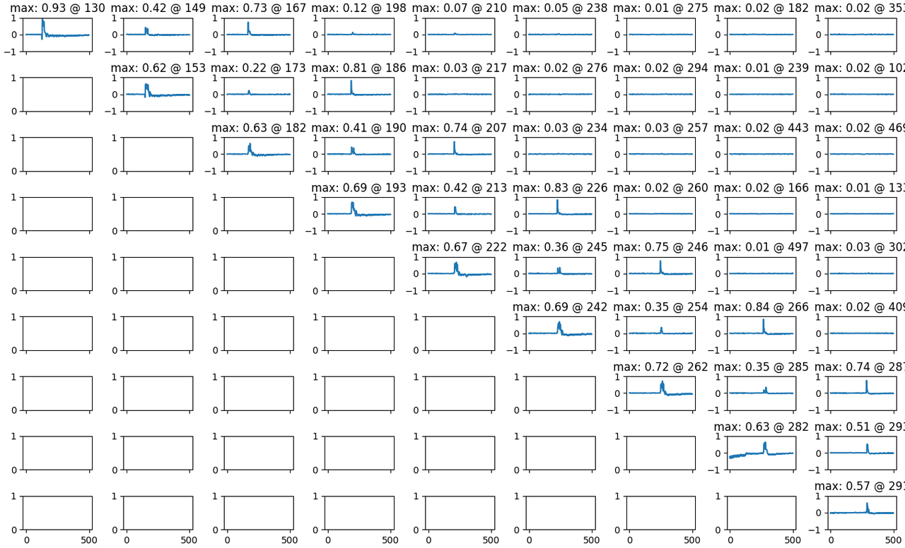
the most correlated relation with respect to the input. And something interesting come out: obviously the
majority of samples have no correlation with nothing, in a couple of points
there is correlation with the input bytes but specific samples (corresponding
to the instruction ld r25, Z+, i.e. the instruction loading the hardcoded
password into a register) correlate to the password!
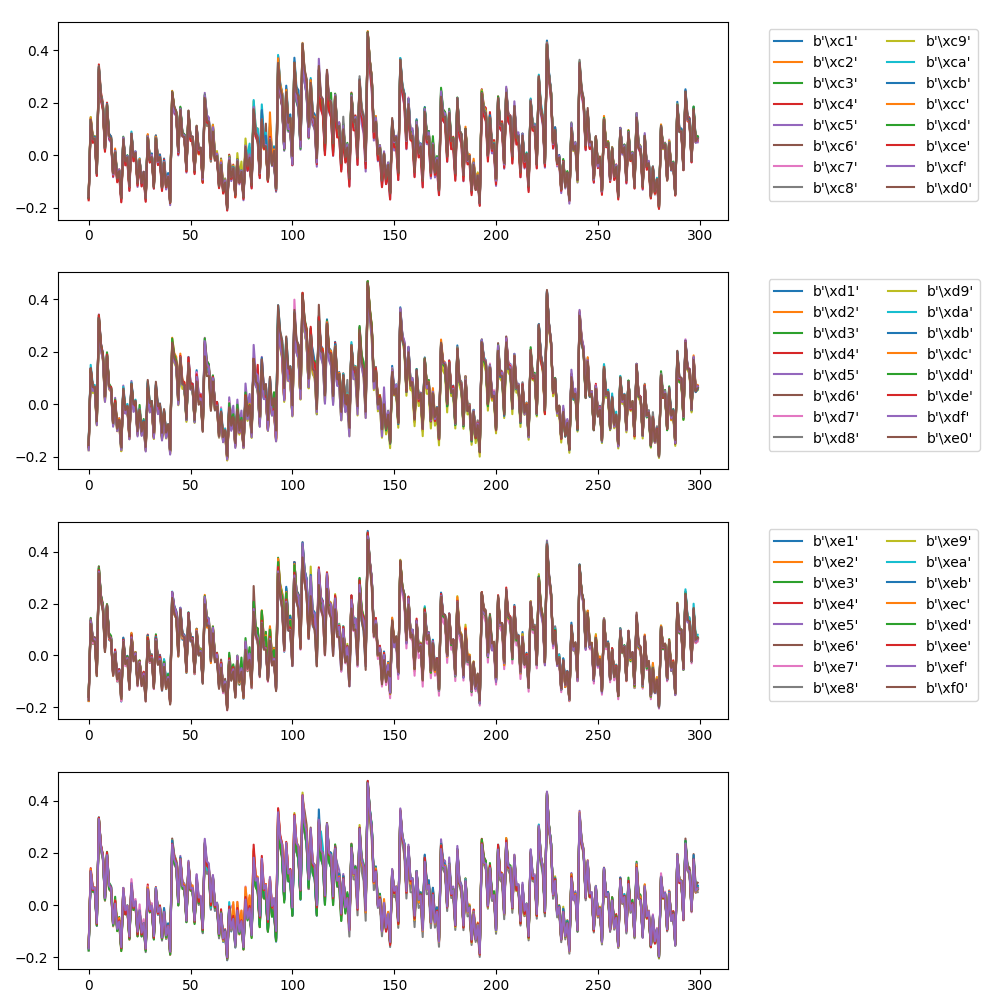
Here the results where each entry is the best correlation between the i-th input byte (row) and the j-th iteration of the instruction (column):
| 0 | 1 | 2 | 3 | 4 | |
|---|---|---|---|---|---|
| 0 | b'k':0.73 | b'\xeb':0.26 | b'\xd4':0.06 | b'\xfe':0.05 | b'\xd6':0.04 |
| 1 | b'F':0.02 | b'e':0.76 | b'\xe5':0.25 | b'\xde':0.07 | b'\xda':0.06 |
| 2 | b'\xbb':0.02 | b'z':0.01 | b'b':0.78 | b'\xe2':0.25 | b'\xbd':0.06 |
| 3 | b'\xbf':0.11 | b'\x9f':0.10 | b'\xbf':0.06 | b'a':0.80 | b'\xe1':0.20 |
| 4 | b']':0.02 | b'\xf7':0.01 | b'v':0.01 | b'\xdf':0.02 | b'b':0.81 |
and the diagonal contains the password (the floating point number is the value of the correlation). For completness here the table with the iterations along the rows and the (eight) samples related to the instruction along the columns
| sample index | 0 | 1 | 2 | 3 | 4 | 5 | 6 | 7 |
|---|---|---|---|---|---|---|---|---|
| 44 | b'\x00' 0.56 | b'+' 0.68 | b'+' 0.73 | b'k' 0.72 | b'k' 0.71 | b'+' 0.60 | b'+' 0.61 | b'+' 0.58 |
| 92 | b'\x80' 0.20 | b'e' 0.67 | b'e' 0.76 | b'e' 0.76 | b'e' 0.74 | b'e' 0.42 | b'e' 0.40 | b'e' 0.39 |
| 140 | b'A' 0.18 | b'b' 0.72 | b'b' 0.78 | b'b' 0.78 | b'b' 0.76 | b'b' 0.43 | b'b' 0.41 | b'b' 0.39 |
| 188 | b'\x88' 0.13 | b'a' 0.73 | b'a' 0.80 | b'a' 0.80 | b'a' 0.78 | b'a' 0.45 | b'a' 0.44 | b'a' 0.42 |
| 236 | b'@' 0.21 | b'b' 0.76 | b'b' 0.82 | b'b' 0.81 | b'b' 0.80 | b'b' 0.45 | b'b' 0.43 | b'b' 0.41 |
Now with this discovery I would expect to see a symmetric relation with the
ldd r20, X+ instruction: if we have correlation between the input byte
(ldd r20, X+) and the password byte (ldd r25, Z+) in a given iteration I would expect to see a
similar correlation between the password byte and the following iteration input byte but this doesn't happen;
if you look at the table with the most correlated bytes you see that there are
interesting correlation with two previous iteration (sample 129, 177, 225)
| sample index | 0 | 1 | 2 | 3 | 4 | 5 | 6 | 7 |
|---|---|---|---|---|---|---|---|---|
| 32 | b'\xb1' 0.01 | b'\x03' 0.82 | b'\x03' 0.87 | b'\x03' 0.86 | b'\x03' 0.83 | b'\x00' 0.90 | b'\x00' 0.91 | b'\x00' 0.90 |
| 80 | b'm' 0.01 | b'\xa1' 0.82 | b'\xa1' 0.88 | b'\xa1' 0.87 | b'\xa1' 0.85 | b'\x80' 0.64 | b'\x80' 0.67 | b'\x80' 0.66 |
| 128 | b'\x15' 0.01 | b'k' 0.78 | b'k' 0.85 | b'k' 0.83 | b'k' 0.81 | b'\x00' 0.44 | b'\x80' 0.49 | b'\x80' 0.49 |
| 176 | b'\x9f' 0.09 | b'e' 0.82 | b'e' 0.88 | b'e' 0.87 | b'e' 0.85 | b'\x00' 0.50 | b'\x00' 0.55 | b'\x80' 0.54 |
| 224 | b'\xf7' 0.01 | b'b' 0.79 | b'b' 0.86 | b'b' 0.84 | b'b' 0.82 | b'\x00' 0.52 | b'\x80' 0.55 | b'\x80' 0.55 |
To summarize the relationship between power consumption and input bytes I'm using the following diagram where in the entry \(\left(i, j\right)\) of the "matrix" you have the correlation with \(I[i]\otimes I[j]\), with \(I[\alpha]\) indicating the \(\alpha\)-th input byte. In the diagonal \(\left(a, a\right)\) instead I placed the direct correlation with the input byte \(I[a]\)
It's possible to see a correlation between two adjacent lds from memory.
Improving the experiment a little, it's possible to manually craft some assembly to unroll the loop in a way that the loadings of the password and the input bytes are not more one after the other, but instead the password is loaded into some registers at the start of the routine (this time I used a different password: "armedilzo", so I don't have repeated characters and is longer)
 75a:   80 93 05 06     sts 0x0605, r24 ; 0x800605 <__TEXT_REGION_LENGTH__+0x7de605>
 75e:   00 e0           ldi r16, 0x00   ; 0
 760:   d9 a0           ldd r13, Y+33   ; 0x21
 762:   fa a0           ldd r15, Y+34   ; 0x22
 764:   1b a1           ldd r17, Y+35   ; 0x23
 766:   ac a1           ldd r26, Y+36   ; 0x24
 768:   ed a1           ldd r30, Y+37   ; 0x25
 76a:   6e a1           ldd r22, Y+38   ; 0x26
 76c:   4f a1           ldd r20, Y+39   ; 0x27
 76e:   28 a5           ldd r18, Y+40   ; 0x28
 770:   89 a5           ldd r24, Y+41   ; 0x29
 772:   e9 80           ldd r14, Y+1    ; 0x01
 774:   de 24           eor r13, r14
 776:   0d 29           or  r16, r13
 778:   ea 80           ldd r14, Y+2    ; 0x02
 77a:   fe 24           eor r15, r14
 77c:   0f 29           or  r16, r15
 77e:   eb 80           ldd r14, Y+3    ; 0x03
 780:   1e 25           eor r17, r14
 782:   01 2b           or  r16, r17
 784:   ec 80           ldd r14, Y+4    ; 0x04
 786:   ae 25           eor r26, r14
 788:   0a 2b           or  r16, r26
 78a:   ed 80           ldd r14, Y+5    ; 0x05
 78c:   ee 25           eor r30, r14
 78e:   0e 2b           or  r16, r30
 790:   ee 80           ldd r14, Y+6    ; 0x06
 792:   6e 25           eor r22, r14
 794:   06 2b           or  r16, r22
 796:   ef 80           ldd r14, Y+7    ; 0x07
 798:   4e 25           eor r20, r14
 79a:   04 2b           or  r16, r20
 79c:   e8 84           ldd r14, Y+8    ; 0x08
 79e:   2e 25           eor r18, r14
 7a0:   02 2b           or  r16, r18
 7a2:   e9 84           ldd r14, Y+9    ; 0x09
 7a4:   8e 25           eor r24, r14
 7a6:   08 2b           or  r16, r24
 7a8:   01 11           cpse    r16, r1
 7aa:   ff cf           rjmp    .-2         ; 0x7aa <main+0xe4>
this time the correlation between two-lds-apart is more apparent.
probably the branch instruction interferes with the lds in some obscure way.
This breaks my method of recovering the password but maybe something can be done for this and if something interesting come up I will tell you in future.
Conclusion
In this post I gave you an overview of what is possible to "see" via power analysis and some of the tools available for it. Maybe I uncovered a new "primitive" to steal secret in chips of the AVR family. Probably there will be a future post about some "advanced" experiments, like capturing traces via an oscilloscope, align them via fourier transform and more.
Linkography
- AVR instruction set manual
- Statistics and Secret Leakage
-
Power Analysis, What Is Now Possible..., paper from
ASIACRYPT2000 - Investigations of Power Analysis Attacks on Smartcards
- Differential Power Analysis, paper by Paul Kocher
- Correlation Power Analysis with a Leakage Model paper introducing the CPA in 2004
- Tamper Resistance - a Cautionary Note
- Understanding Power Trace, post from NewAE forum explaining the meaning of the power traces
- CHIP.FAIL – GLITCHING THE SILICON OF THE CONNECTED WORLD
-
Fault diagnosis and tolerance in cryptography (FDTC) 2014 with some slides:
- https://fdtc.deib.polimi.it/FDTC11/shared/FDTC-2011-session-4-3.pdf
- https://fdtc.deib.polimi.it/FDTC11/shared/FDTC-2011-session-2-1.pdf
- https://fdtc.deib.polimi.it/FDTC14/shared/FDTC-2014-session_1_1.pdf
- POWER ANALYSIS BASED SOFTWARE REVERSE ENGINEERING ASSISTED BY FUZZING II
- Power Analysis For Cheapskates
- Side-channel Attacks Using the Chipwhisperer
- Pearson's correlation
-
For an extensive explanation you can use the book "Nanometer CMOS ICs, From Basics to ASICs" pg 161 ↩
-
Optimal statistical power analysis; E. Brier, C. Clavier, F. Olivier (link to the paper) ↩↩
-
Hacker's delight pg95 and pg343 ↩
Comments
Comments powered by Disqus