Selecting random points on a triangle

2025-12-20

Gianluca Pacchiella

Tags:

In this blog post the author explains a couple of ways to choose uniformly a point from a triangle and the first approach that he uses is via the barycentric coordinate: given a triangle identified by the three points $A$, $B$ and $C$

Generate three random numbers $\alpha$, $\beta$ and $\gamma$ using a uniform distribution from the interval $[0, 1]$
Normalize the point in such a way that they have sum equal to 1
use $\alpha A + \beta B + \gamma C$ as the chosen point

The resulting points are not actually uniformly distributed, fact acknowledged by the author itself simply showing a plot of the distribution of the points, my problem is that a plot is not a proof, so this post will try to fix that!

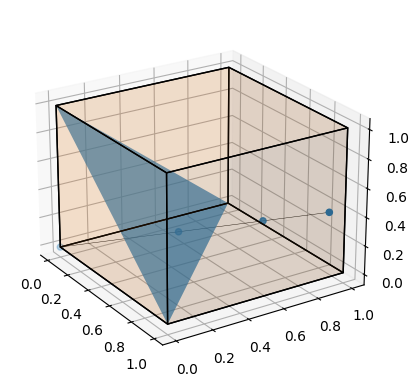
Let me start saying that geometrically, the choice of the three random numbers at step one is the same as selecting one random point inside a unit cube.

Then the normalization at step two is the same as projecting the point into the 2-simplex represented by the triangle with vertices of the cube with a single $1$ in their coordinates.

If we create a line connecting the origin to the selected point and we prolong it until it reaches the boundary of the cube (i.e. a face or an edge) we obtain all the points that identifies as the representative point on the simplex and the length of such segment is not constant, explaining the reason of why is not uniform.

(With this post I'm going to try embedding python in the actual page using pyodide, marimo and webassembly; click the button to activate the two notebooks, but be aware that is going to load ~100MB of external data; here a marimo notebook with similar calculations).

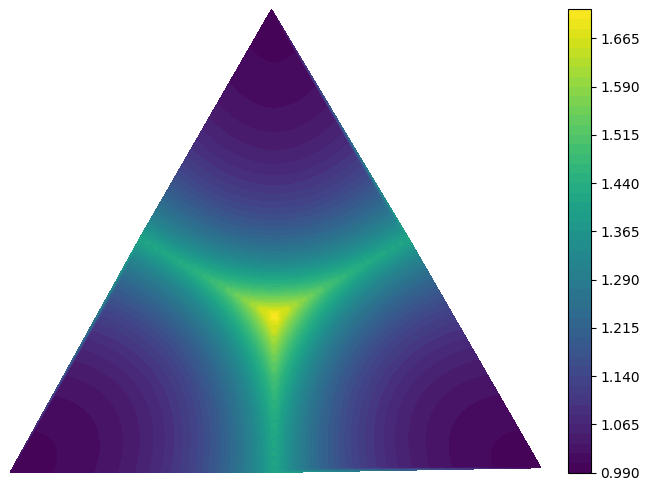
To calculate such length suppose we have the coordinate of the point that is on the boundary, suppose that is the top face of the cube with coordinate $\left(\hat\lambda_1, \hat\lambda_2, 1\right)$ this corresponds to a mapping to the normalized point on the simplex

$$ \left(\hat\lambda_1, \hat\lambda_2, 1\right) \rightarrow \left(\lambda_1 = {\hat\lambda_1\over 1 + \hat\lambda_1 + \hat\lambda_2}, \lambda_2 = {\hat\lambda_2\over 1 + \hat\lambda_1 + \hat\lambda_2}, \lambda_3 = {1\over 1 + \hat\lambda_1 + \hat\lambda_2}\right) $$

the length of the segment is $L(\hat\lambda_1, \hat\lambda_2) = \sqrt{1 + \hat\lambda^2_1 + \hat\lambda_2^2}$, (we are using the pythagorean theorem where one side is the $\lambda_3$ axis and the other is the segment from the corner of the cube to the point hitting the boundary).

We realize that $\lambda_1 = \hat\lambda_1\lambda_3$, so that we can rewrite the relationship in the following way

$$ \left\{\eqalign{ \hat\lambda_1 &= {\lambda_1\over\lambda_3}\cr \hat\lambda_2 &= {\lambda_2\over\lambda_3}\cr }\right. $$

(it's fascinating how this mimics the projection of the complex plane into the sphere); now if we rewrite the length of the segment in the barycentric coordinates we obtain $$ L_3(\lambda_1, \lambda_2, \lambda_3) = \sqrt{1 + {\lambda^2_1 + \lambda_2^2\over\lambda^2_3}}\,\hbox{when}\,\,\lambda_3 \gt {1\over3},\, \lambda_1\lt\lambda_3,\, \lambda_2\lt\lambda_3 $$

Now you can assume that the other three sections of the simplex have a functionally identical formula, where you permutate the barycentric coordinates labels.

import marimo as mo
import random
import math

import matplotlib.pyplot as plt
from matplotlib import colormaps
from mpl_toolkits.mplot3d.art3d import Poly3DCollection
import numpy as np

triangle = np.array([[0, 0], [1, 0], [1/2, np.sin(np.pi/3)], [0, 0]])

def rotate(xy, center, radians):
    """Use numpy to build a rotation matrix and take the dot product."""

    c, s = np.cos(radians), np.sin(radians)
    j = np.matrix([[c, s], [-s, c]])
    m = j@(xy - center)

    return np.array(m.ravel().T)[:,0] + center

def rotate_wrt_simplex_center(xy, radians):
    center = b2p(1/3, 1/3, 1/3)
    return rotate(xy, center, radians)

def b2p(alpha, beta, gamma):
    return alpha*triangle[0] + beta*triangle[1] + gamma*triangle[2]

def value(alpha, beta, gamma):
    return math.sqrt(1 + (alpha**2 + beta**2)/gamma**2)

def rotate_XY(xy):
    rrr = lambda _:rotate_wrt_simplex_center(_, 2*np.pi/3)
    return np.array(list(map(rrr, xy)))

# create a function otherwise too much pollution with variables
def weights():
    """Generate the data to plot a 3d visualization of the weights."""
    # t1, t2, t3 don't have equal dimensions so we cannot create a tensor
    # out of it, instead we are going to create a 2d array from the resulting
    # 2d coordinates
    xyz = []
    # start with t1 equal to 1, so we loop over what we remove from it
    for extra in range(100):
        for t2 in range(0, extra):
            t1 = (100 - extra)/100
            t2 = t2/100
            t3 = 1 - t1 - t2

            if not (t3 > 1/3 and t1 <= t3 and t2 <= t3):
                continue

            p = b2p(t1, t2, t3)
            v = value(t1, t2, t3)
            xyz.append(np.append(p, v))

    xyz = np.array(xyz)

    return xyz


xyz = weights()
fig0, ax0 = plt.subplots(subplot_kw=dict(projection='3d'))
surf = ax0.scatter(*xyz.T, c=xyz[...,2], s=2, cmap=colormaps['plasma'])

XYZ = np.copy(xyz)
XYZ[...,0:2] = rotate_XY(XYZ[...,0:2])
surf = ax0.scatter(*XYZ.T, c=XYZ[...,2], s=2, cmap=colormaps['plasma'])

XYZ2 = np.copy(XYZ)
XYZ2[...,0:2] = rotate_XY(XYZ2[...,0:2])
surf = ax0.scatter(*XYZ2.T, c=XYZ2[...,2], s=2, cmap=colormaps['plasma'])

#plt.show()
mo.mpl.interactive(plt.gcf())

final = np.concatenate((xyz, XYZ, XYZ2), axis=0)
fig_contour, ax_contour = plt.subplots(layout='constrained')
CS4 = ax_contour.tricontourf(*final.T, 50, extend3d=True)
fig_contour.colorbar(CS4)
ax_contour.set_axis_off()
#plt.show()

mo.mpl.interactive(plt.gcf())

Comments